happign for forester
Paul Carteron
2025-07-23
Source:vignettes/articles/happign_for_foresters.Rmd
happign_for_foresters.Rmd
knitr::opts_chunk$set(
  collapse = TRUE,
  out.width = "100%",
  dpi = 300,
  fig.width = 7.2916667,
  comment = "#>"
)First choose a zone of interest
For the example we will work with the Camors forest. First of all we
need the commune border that can be obtained with
get_apicarto_cadastre() from the insee code. For
convenience, happign provides a table containing all insee
codes (data("com_2025")).
data("com_2025", package = "happign")

#search communes name Camors and extract insee code
insee_code <- com_2025[grepl("^Camors", com_2025$LIBELLE_COM),"COM"]

camors <- get_apicarto_cadastre(insee_code, type = "commune")

tm_shape(camors)+
   tm_borders()+
   tm_text("nom_com")
An other way of getting borders without Apicarto is to use ECQL language to directly query IGN WFS geoservers.
camors2 <- get_wfs(
   layer = "ADMINEXPRESS-COG-CARTO.LATEST:commune",
   query = "nom_officiel_en_majuscules LIKE 'CAMORS'"
)

# "nom_officiel_en_majuscules" attribut can be found using get_wfs_attributes(layer = "ADMINEXPRESS-COG-CARTO.LATEST:commune")
Download cadastral parcel
Cadastral parcels are essential for any forest manager. Here how to
download it with get_apicarto_cadastre. We will work only
on section "H".
camors_parcels <- get_apicarto_cadastre(insee_code, type = "parcelle", section = "H")

tm_shape(camors_parcels)+
   tm_polygons(fill_alpha = 0, lwd = 0.5)+
tm_shape(camors)+
   tm_borders(col = "red", lwd = 2)
Rq :
- IGN WFS can return a maximum of 1000 features. The
get_wfs()function overrides this limit by performing several consecutive requests as the console show
Downloading BD Forêt
The first interesting layer for forester is the “BD Forêt” which is all vegetation type assigned to each area greater than or equal to 0.5 ha (5,000 m²). There is two layer for forest : the old one BD Forêt V1 and the new one BD Forêt V2 that can be accessed with “burger menu” on the top left of interactive map below.
layer_v1 <- "LANDCOVER.FORESTINVENTORY.V1:resu_bdv1_shape"
bd_foret_v1 <- get_wfs(camors, layer_v1, predicate = intersects())
#> ⠙ iterating 1 done (0.46/s) | 2.2s
#> iterating ■■■■■■■■■■■■■■■■■■■■■■■■■■■■■■■  100% | ETA:  0s

layer_v2 <- "LANDCOVER.FORESTINVENTORY.V2:formation_vegetale"
bd_foret_v2 <- get_wfs(camors, layer_v2, predicate = intersects())

tm_shape(bd_foret_v1) +
   tm_polygons(fill = "libelle",
               popup.vars = names(bd_foret_v1)[1:(ncol(bd_foret_v1)-2)],
               fill.legend = tm_legend_hide())+
tm_shape(bd_foret_v2) +
    tm_polygons(fill = "tfv",
                fill_alpha = 0.5,
                popup.vars = names(bd_foret_v2)[1:(ncol(bd_foret_v2)-2)],
                fill.legend = tm_legend_hide()) +
tm_shape(camors) +
   tm_borders(lwd = 2)
More calculations can be done to get a better understanding of forest type. Below, areas per species are calculated :
bd_foret_v2$area <- as.numeric(st_area(bd_foret_v2) / 10000)

# Aggregate by essence
species <- aggregate(
  area ~ essence,
  data = bd_foret_v2,
  sum
)

# Reorder factor levels by decreasing area
species$essence <- factor(
  species$essence,
  levels = species$essence[order(species$area, decreasing = TRUE)]
)

ggplot() +
  geom_col(
    data = species,
    aes(
      x = essence,
      y = area,
      fill = essence
    )
  ) +
  theme_bw() +
  labs(
    title = "Surface couverte par essences [ha]",
    y = "Surface [ha]",
    x = "",
    fill = "Essence :"
  ) +
  theme(axis.text.x = element_blank())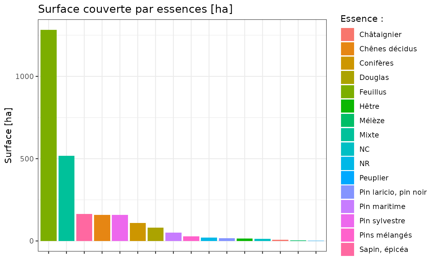
Detect protected area
One information you really want when you’re a forest manager is if your zone of interest is inside protected area. You can for exemple, test for all layer containing “PROTECTED” so you can be sure that you have all of them. In the example code below i only search for ZNIEFF.
Again, you can click on map, point and shape for more informations.
wfs <- get_layers_metadata("wfs")
znieff_layers <- wfs$Name[grepl("ZNIEFF", wfs$Name, ignore.case = TRUE)]

znieff <- lapply(
   znieff_layers,
   function(layer){get_wfs(camors, layer)}
)
names(znieff) <- znieff_layers

# remove empty layers
znieff <- Filter(function(x) nrow(x) >= 1 , znieff)

# Plot the result
tm_shape(camors) +
   tm_borders(lwd = 2)+
tm_shape(znieff[[1]])+
   tm_polygons(fill_alpha = 0.8, col = "blue")
MNS, MNT and MNH…
Terrain topologie is quite useful for forest management. IGN offers MNT and MNS for download. As a reminder, the MNT corresponds to the surface of the ground and the MNS to the real surface (in our case, the trees). It is thus easy to find the height of the trees by subtracting the MNT from the MNS.
mnt_layer <- "ELEVATION.ELEVATIONGRIDCOVERAGE.HIGHRES"
mnt <- get_wms_raster(camors_parcels, mnt_layer, res = 10, crs = 2154, rgb = FALSE)
#> 0...10...20...30...40...50...60...70...80...90...100 - done.
#> Warp executed successfully.

mns_layer <-"ELEVATION.ELEVATIONGRIDCOVERAGE.HIGHRES.MNS"
mns <- get_wms_raster(camors_parcels, mns_layer, res = 10, crs = 2154, rgb = FALSE)
#> 0...10...20...30...40...50...60...70...80...90...100 - done.
#> Warp executed successfully.

# Calculate digital height model i.e. tree height
mnh <- mns - mnt
mnh[mnh < 0] <- NA  # Remove negative value
mnh[mnh > 50] <- 40 # Remove height more than 50m

# tmap v4 code
tm_shape(mnh) +
  tm_raster(
     col.scale = tm_scale_continuous(values = "carto.earth", value.na = "grey"),
     col.legend = tm_legend(title = "Height", showNA = F)
) +
tm_shape(camors_parcels, is.main = TRUE)+
   tm_borders() +
tm_shape(camors)+
   tm_borders(lwd = 2, col = "firebrick")
#> Warning: tm_scale_intervals `label.style = "continuous"` implementation in view mode
#> work in progress
NDVI
The code below present the calculation of the NDVI. All informations and palette come from this website The value range of an NDVI is -1 to 1. It is (Near Infrared - Red) / (Near Infrared + Red) :
- Water has a low reflectance in red, but almost no NIR (near infrared) reflectance. So the difference will be small and negative, and the sum will be small, and NDVI large and negative.
- Plants have a low reflectance in red, and a strong NIR reflectance. So the difference will be large and positive, and the sum will be just about the same as the difference, so NDVI will be large and positive.
Categories are somewhat arbitrary, and you can find various rules of thumb, such as:
- Negative values of NDVI (values approaching -1) correspond to water. Values close to zero (-0.1 to 0.1) generally correspond to barren areas of rock, sand, or snow. Low, positive values represent shrub and grassland (approximately 0.2 to 0.4), while high values indicate temperate and tropical rainforests (values approaching 1).
- Very low values of NDVI (0.1 and below) correspond to water, barren areas of rock, sand, or snow. Moderate values represent shrub and grassland (0.2 to 0.3), while high values indicate temperate and tropical rainforests (0.6 to 0.8).
# In fact IRC have 80cm resolution, but to avoid too slow ploting, res = 5 is used
# I also add a buffer to have more than the area
irc <- get_wms_raster(st_buffer(camors_parcels, 500),
                      res = 5,
                      layer = "ORTHOIMAGERY.ORTHOPHOTOS.IRC")
#> 0...10...20...30...40...50...60...70...80...90...100 - done.
#> Warp executed successfully.

# calculate ndvi from near_infrared and infrared
ndvi_fun <- function(nir, red){
  (nir - red) / (nir + red)
}

ndvi <- lapp(irc[[c(1, 2)]], fun = ndvi_fun)

# palette for plotting
breaks_ndvi <- c(-1,-0.2,-0.1,0,0.025 ,0.05,0.075,0.1,0.125,0.15,0.175,0.2 ,0.25 ,0.3 ,0.35,0.4,0.45,0.5,0.55,0.6,1)
palette_ndvi <- c("#BFBFBF","#DBDBDB","#FFFFE0","#FFFACC","#EDE8B5","#DED99C","#CCC782","#BDB86B","#B0C261","#A3CC59","#91BF52","#80B347","#70A340","#619636","#4F8A2E","#407D24","#306E1C","#216112","#0F540A","#004500")


#tmap v4 code
tm_shape(ndvi)+
   tm_raster(
      col.scale = tm_scale_continuous(
         limits = c(-1, 1),
         values = palette_ndvi,
      ),
      col.legend = tm_legend(title = "NDVI")
      )+
tm_shape(camors_parcels, is.main = TRUE)+
   tm_borders(lwd = 2, col = "blue")
#> Warning: tm_scale_intervals `label.style = "continuous"` implementation in view mode
#> work in progress
The gloss index
The gloss index represents the average of the image glosses. This index is therefore sensitive to the brightness of the soil, related to its moisture and the presence of salts on the surface. It characterizes especially the albedo (solar radiation that is reflected back to the atmosphere). The gloss index allows us to estimate whether the observed surface feature is light or dark.
# calculate gloss_index from near_infrared and infrared
gloss_fun <- function(nir, red){
  sqrt(red^2 + nir^2)
}

gloss_index <- lapp(irc[[c(1, 2)]],
            fun = gloss_fun)

# tmap v4 code
tm_shape(gloss_index)+
   tm_raster(col.legend = tm_legend(title = "GLOSS INDEX"))+
tm_shape(camors_parcels, is.main = TRUE)+
   tm_borders(lwd = 2, col = "blue")
Last but not least… BD Topo
BD topo from IGN covers in a coherent way all the geographical and administrative entities of the national territory. So you can find in it :
- Administrative (boundaries and administrative units);
- Addresses (mailing addresses) ;
- Building (constructions) ;
- Hydrography (water-related features) ;
- Named places (place or locality with a toponym describing a natural space or inhabited place);
- Land use (vegetation, foreshore, hedge);
- Services and activities (utilities, energy storage and transportation, industrial sites);
- Transportation (road, rail or air infrastructure, routes);
- Regulated areas (most of the areas are subject to specific regulations).
For the example below I choose to download all water-related data :
cour_eau <- get_wfs(camors, "BDTOPO_V3:cours_d_eau", intersects())
detail_hydro <- get_wfs(camors, "BDTOPO_V3:detail_hydrographique", intersects())
surf_hydro <- get_wfs(camors, "BDTOPO_V3:surface_hydrographique", intersects()) # water detected by satellite

tm_shape(camors)+
   tm_borders(lwd = 2)+
tm_shape(cour_eau)+
   tm_lines(col = "blue")+
tm_shape(detail_hydro)+
   tm_dots(col = "red")+
tm_shape(surf_hydro)+
   tm_polygons("steelblue")