Before starting
We can load the happign package, and some additional
packages we will need (sf to manipulate spatial data and
tmap to create maps)
WFS, WMS, and WMTS services
happign provides access to three web services published
by IGN (Institut national de l’information géographique
et forestière):
WFS (Web Feature Service): Vector data (points, lines, polygons)
WMS (Web Map Service): Raster images generated on the fly
WMTS (Web Map Tile Service): Raster map images served as pre-generated tiles, optimized for fast display.
The official OGC specifications for these services are available online:
How to download data with happign
To retrieve data using happign, two pieces of
information are required:
What to download: The name of the layer exposed by the IGN service (acces with
get_layers_metadata())Where to download it: An area of interest, provided as an
sfgeometry (from the{sf}package).
happign then takes care of building the web service
requests and returns data usable in R.
Layer names
Layer names can be obtained directly from the IGN website. For
example, in the WFS service, the first layer listed in
the Administratif
category is:
"ADMINEXPRESS-COG-CARTO.LATEST:arrondissement"
To avoid copying layer names manually, happign provides
the get_layers_metadata() function, which queries the IGN
services directly and always returns the most up-to-date list of
available layers.
This function can be used with WFS, WMS, and WMTS services:
wfs_layers <- get_layers_metadata(data_type = "wfs")
wms_layers <- get_layers_metadata(data_type = "wms-r")
wmts_layers <- get_layers_metadata(data_type = "wmts")
The returned object contains metadata for each available layer, including name, title, and service-specific information.
Downloading data
After selecting layer name, downloading data with
happign only requires a few lines of code.
In the following example, we focus on the town of
Penmarc’h (France). A polygon representing part of this
municipality is included in happign and will be used as the
area of interest.
penmarch <- sf::read_sf(system.file("extdata/penmarch.shp", package = "happign"))WFS ; vector data
The get_wfs() function is used to download vector data
from IGN WFS services.
In this first example, we retrieve the administrative boundaries of Penmarc’h.
penmarch_borders <- get_wfs(
  x = penmarch,
  layer = "LIMITES_ADMINISTRATIVES_EXPRESS.LATEST:commune"
)
# Plotting result
tm_shape(penmarch_borders) +
  tm_polygons() +
  tm_add_legend(
    type = "polygons",
    position = c("right", "top"),
    labels = "Penmarc’h borders from `get_wfs()`"
  ) +
  tm_shape(penmarch) +
  tm_polygons(fill = "red") +
  tm_add_legend(
    type = "polygons",
    fill = "red",
    position = c("right", "top"),
    labels = "`penmarch` shape from `happign`"
  ) +
  tm_title(
    "Penmarc’h administrative boundaries (IGN)",
    position = tm_pos_out("center", "top", pos.h = "center")
  )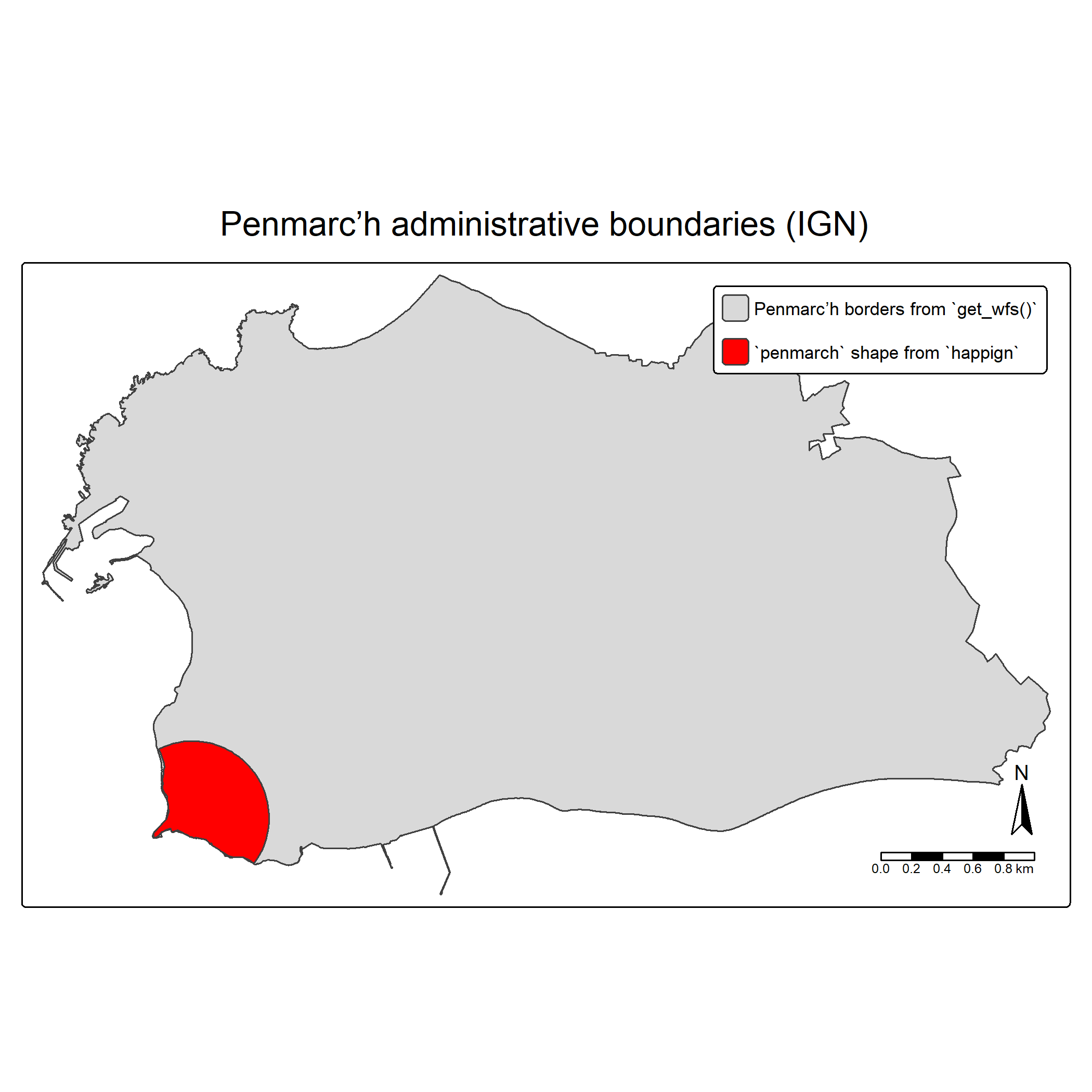
That is all it takes to retrieve vector data using WFS !
From there, you can explore the wide range of datasets provided by IGN. For instance, you may wonder how many roundabout are recorded in Penmarc’h (Spoiler: there are 8 of them!)
WFS & predicate:
In the example below, spatial predicate is used to refined the query
using the argument predicate. The goal is to download only
roundabout entirely contained within the Penmarc’h so
within() predicate is used.
Default predicate is bbox() (generally fastest). All
available are documented in ?spatial_predicates :
intersects(), within(),
disjoint(), contains(),
touches(), crosses(), overlaps(),
equals(), bbox(), dwithin(),
beyond(), relate().
roundabout <- get_wfs(
  x = penmarch_borders,
  layer = "BDCARTO_V5:rond_point",
  predicate = within()
)
# Plotting result
tm_shape(penmarch_borders) +
  tm_polygons() +
  tm_add_legend(
    type = "polygons",
    position = c("right", "top"),
    labels = "Penmarc’h borders from `get_wfs()`"
  ) +
tm_shape(roundabout) +
  tm_symbols(fill = "firebrick", lwd = 2) +
  tm_add_legend(
    type = "symbols",
    fill = "firebrick",
    position = c("right", "top"),
    labels = "Roundabout"
  ) +
  tm_title(
    "Roundabout recorded by IGN in Penmarc’h",
    position = tm_pos_out("center", "top", pos.h = "center")
  )
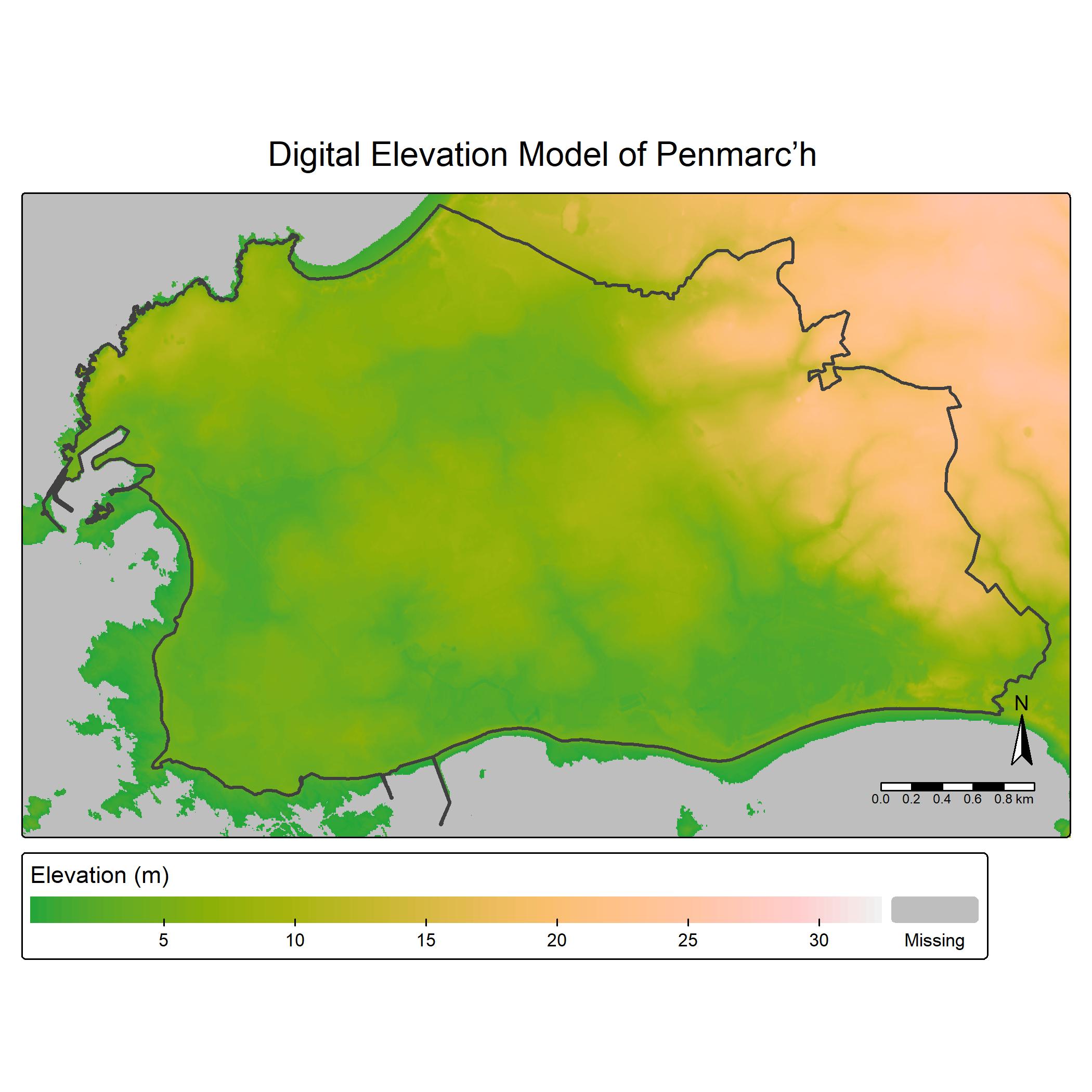
WMS raster
For raster data, the workflow is very similar, but relies on the
get_wms_raster() function. In addition to the layer name,
you must specify a spatial resolution.
Note that the resolution must be expressed in the same coordinate
reference system as the crs parameter.
The Altimétrie category provides several elevation-related datasets. A common example is the Digital Elevation Model (DEM).
In the example below, the administrative boundaries of Penmarc’h are
used to download a DEM. For elevation data, we are interested in numeric
pixel values rather than RGB colors, which is why
rgb = FALSE is used.
layers_metadata <- get_layers_metadata("wms-r", "altimetrie")
dem_layer <- layers_metadata[3, 1] # ELEVATION.ELEVATIONGRIDCOVERAGE.HIGHRES

mnt <- get_wms_raster(
  x = st_buffer(penmarch_borders, 800),
  layer = dem_layer,
  res = 5,
  crs = 2154,
  rgb = FALSE
)
#> 0...10...20...30...40...50...60...70...80...90...100 - done.
#> Warp executed successfully.

# Remove negative values (possible edge artefacts)
mnt[mnt < 0] <- NA
tm_shape(mnt) +
  tm_raster(
    col.scale  = tm_scale_continuous(values = "terrain", value.na = "grey"),
    col.legend = tm_legend(title = "Elevation (m)", orientation = "landscape")
  ) +
tm_shape(penmarch_borders, is.main = TRUE) +
  tm_borders(lwd = 2) +
  tm_title(
    "Digital Elevation Model of Penmarc’h",
    position = tm_pos_out("center", "top", pos.h = "center")
  )
Note: Rasters returned by get_wms_raster() are
SpatRaster objects from the terra package.
For an overview of raster class conversions in R, see: https://geocompx.org/post/2021/spatial-classes-conversion/
WMTS
For WMTS services, no spatial resolution needs to be specified because the images are pre-generated. Instead, a zoom level must be provided. Higher zoom levels correspond to finer spatial detail and higher visual quality.
When the goal is visualization rather than quantitative analysis, WMTS is generally preferable to WMS, as it is faster and better suited for map display.
layers_metadata <- get_layers_metadata("wmts", "ortho")
ortho_layer <- layers_metadata[1, 3] # ORTHOIMAGERY.ORTHOPHOTOS
tiny_penmarch <- read_sf(system.file("extdata/penmarch.shp", package = "happign"))

hr_ortho <- get_wmts(
  x = tiny_penmarch,
  layer = ortho_layer,
  zoom = 9
)
tm_shape(hr_ortho) +
  tm_rgb() +
  tm_shape(penmarch_borders) +
  tm_borders(lwd = 2, col = "white") +
  tm_title(
    "Orthophoto",
    position = tm_pos_out("center", "top", pos.h = "center")
  )
WMTS layers are ideal for background maps, orthophotography, and any use case where visual clarity and performance are more important than direct access to raw pixel values.